Sunday, 10 January 2016
Slıde Show
You can show my ppt slıde show
https://drive.google.com/open?id=0BzOux6K933t5SUJpYUJRQlRsODg
https://drive.google.com/open?id=0BzOux6K933t5SUJpYUJRQlRsODg
6 things all engineers should know before using FEA
6 things all engineers should know before using FEA
Engineers in every industry are integrating finite element analysis (FEA) into the design cycle to ensure that their products are safe, cost-effective, and fast to market. But, analysis is not as simple as putting a CAD model into any FEA package.
There are more software options today than ever before. For many years, engineers were limited to using linear static stress analysis. More recently, finite element packages have been extended to include nonlinear static stress, dynamic stress (vibration), fluid flow, heat transfer, electrostatic, and FEA-based stress and motion analysis capabilities. These capabilities are frequently combined to perform analyses that consider multiple physical phenomena, and are tightly integrated within a CAD interface.
This article will briefly discuss some FEA basics and then outline what engineers need to know when they decide to use FEA.
1. FEA basics. A finite element model is a discrete representation of the continuous, physical part being analyzed. This representation is created using nodes, which are connected together to form elements. The nodes are the discrete points on the physical part where the analysis will predict the response of the part due to applied loading. This response is defined in terms of nodal degrees of freedom (DOF). For stress analysis, up to six degrees of freedom are possible at each node (three components of translation and three components of rotation), depending on the element type selected (e.g., beam, plate, 2D, and 3D elements).
The grid of connecting elements at common nodes comprises the mesh. When adjacent elements share nodes, the displacement field is continuous across the shared element boundary and loads can be transferred between the elements.
2. Design criteria. In any analysis, an engineer first needs to determine the significant physical phenomena and environmental conditions to which the part will be exposed, and also the desired design objective. For example, one of the most common concerns for engineers involves maximizing the part's durability.
The first step in an analysis is to determine whether the design will be subject to static or dynamic conditions. In its real-world application, is the part fixed in space, subject to vibration, or does it move relative to other parts in the assembly? What happens when you run the entire product through its motion cycle? For years, engineers faced with expensive computing resources have simplified the problem by using static FEA software to calculate stresses at a single instant in time. This method works only if the design does not experience impact, motion, or changes in applied loads over time.
3. Multiphysics. In addition to considering a part's ability to withstand mechanical stresses, FEA software often enables engineers to predict other real-world stresses, such as: the effects of extreme temperatures or temperature change (heat transfer analysis), the flow of fluids through and around objects (fluid flow analysis), or voltage distributions over the surface or throughout the volume of an object (electrostatic analysis).
Often these effects work in unison, so it is important that the FEA program can consider their effects on one another. For instance, a computer chip may be heating up over time, cooled down by airflow from a fan, vibrated against other parts, and electrically charged. A typical approach might be to isolate and calculate each variable, then feed the results into the FEA program one at a time. Yet each variable could also affect all the others, so either a coupled analysis or tools for relating results is often necessary.
4. Motion simulation. With today's cheaper, faster computers, a growing trend in FEA is the simulation of large-scale motion using finite element models. In the past, the design process demanded specialists who could build models for different uses: design, machining, or analysis. But with more computing power at their fingertips, today's engineers can use the same model for all three demands, and even perform a motion analysis from their desktops. There are three common methods:
Motion Load Transfer requires engineers to use two applications: a kinematics package is used to obtain approximate loads, which are then input to an FEA program for analysis. This approach does not simulate the motion of a finite element model, just many approximate static points. It's faster than calculating stresses by hand, but it uses a rigid-body motion program, so the engineer must accept certain assumptions. For instance, parts like gaskets are flexible, but a rigid-body program can't calculate that.
The Explicit Timestep Method does simulate a model's actual motion, using a huge number of short time intervals. It determines a solution by "marching" along in time, extrapolating from the solution of the prior timestep. This method is fast for a given time interval, but it can take too long for an entire scenario. For example, if you're simulating a car crashing into a telephone pole, it would be impractical with this approach to consider more than the actual moment of impact.
The Implicit Timestep Method and automatic timestepping scheme of FEA-based stress and motion analysis allows for the simulation of a model's motion cycle by running at larger timesteps for periods of relative inactivity, such as a constant acceleration or deceleration, and then automatically reduces the timestep size to capture periods of critical activity, like surface-to-surface contact, local buckling, or impact. Therefore, an accurate solution for the motion, deformation and stresses of a part becomes practical. However, as always, there's some tradeoff of speed for accuracy—since this approach calculates results for every point in time.
5. Modeling. After determining the type of analysis required and the characteristics of the operating environment, the engineer must produce a finite element model with appropriate analysis parameters, such as loads, constraints, and a suitable mesh. The three available methods of CAD/FEA interoperability can vary widely in terms of ease-of-use, accuracy, and functionality:
The CAD universal file format method requires an engineer to export the CAD solid model to a neutral file format, such as IGES, ACIS or Parasolid, and then import the neutral file into the FEA system for setup and analysis. Although this method usually enables engineers to take full advantage of an FEA program, it can also result in the loss of CAD geometry data as the model is translated. So it's not an ideal method, since it sometimes involves using a simplified version of the problem.
The "one window" CAD/FEA method requires no file translation, since the FEA vendor builds analysis capabilities into a CAD solid modeler. Users choose this option for its ease-of-use, as they can access FEA capabilities from a pull-down menu in a single application. However, FEA providers often simplify their one-window versions due to space and interface limitations. In addition, it can also be limited since FEA companies must tailor their product to each CAD vendor's software in order to integrate the two products. So this CAD/FEA interoperability method may require the engineer to purchase and learn other software if he or she is working in a multi-CAD environment or with moderate to advanced analysis capabilities.
The "one window away" CAD/FEA method also requires no file translation, but it has the additional abilities to perform FEA analysis on a different computer from the CAD solid modeler, and to use a single interface for multiple CAD packages. The primary difference is that the FEA runs in a separate application, so an FEA vendor can supply a more complete version (such as including more element types, meshing, and analysis options) without requiring the need for other analysis software. One possible drawback to this approach is that the engineer must learn both the CAD and FEA software.
6. Results interpretation. Once an engineer gets analysis results, he or she inevitably asks, "How do I know my answers are correct?" So FEA software must provide result verification or validation tools. Ideally, these tools would not only include displacement, stress, or other result contours, but also precision contours that provide qualitative and quantitative verification.
Often, the analysis and modeling choices that an engineer makes will determine how easy it is to interpret results. For example, if a linear static stress analysis was performed, only contours at a single instant in time will be available. The stresses displayed will need to be interpreted in some way, such as comparing the values to the yield stress of the material used in the analysis. In addition, the engineer has assumed that the one instant analyzed in the linear static stress analysis represents the worst case scenario.
If, on the other hand, an FEA-based stress and motion analysis was performed on a solid assembly, interpreting the results will be much easier because the model can be seen to move, flex, bend, and even break over time. These time-dependent results can be recorded in an animation file, such as the Windows .avi format.
In addition to animation capabilities, engineers should expect the FEA software to have a fast, easy-to-use visualization tool for reviewing and presenting results for all analysis types with other integrated presentation options, such as automatic options to generate image files of result contours and plots, VRML files, and HTML reports. These tools can be used to prepare a presentation of results to other engineers and even managers and clients.
Carefully considering the analysis, modeling and results interpretation issues discussed here will help engineers to present their designs with more confidence in the validity of their FEA results.
History
While it is difficult to quote a date of the invention of the finite element method, the method originated from the need to solve complex elasticity and structural analysis problems in civil and aeronautical engineering. Its development can be traced back to the work by A. Hrennikoff and R. Courant. In China, in the later 1950s and early 1960s, based on the computations of dam constructions, K. Feng proposed a systematic numerical method for solving partial differential equations. The method was called the finite difference method based on variation principle, which was another independent invention of finite element method. Although the approaches used by these pioneers are different, they share one essential characteristic: mesh discretization of a continuous domain into a set of discrete sub-domains, usually called elements.
Hrennikoff's work discretizes the domain by using a lattice analogy, while Courant's approach divides the domain into finite triangular subregions to solvesecond order elliptic partial differential equations (PDEs) that arise from the problem of torsion of a cylinder. Courant's contribution was evolutionary, drawing on a large body of earlier results for PDEs developed by Rayleigh, Ritz, and Galerkin.
The finite element method obtained its real impetus in the 1960s and 1970s by the developments of J. H. Argyris with co-workers at the University of Stuttgart,R. W. Clough with co-workers at UC Berkeley, O. C. Zienkiewicz with co-workers Ernest Hinton, Bruce Irons and others at the University of Swansea,Philippe G. Ciarlet at the University of Paris 6 and Richard Gallagher with co-workers at Cornell University. Further impetus was provided in these years by available open source finite element software programs. NASA sponsored the original version of NASTRAN, and UC Berkeley made the finite element program SAP IV widely available. In Norway the ship classification society Det Norske Veritas (now DNV GL) developed Sesam in 1969 for use in analysis of ships. A rigorous mathematical basis to the finite element method was provided in 1973 with the publication by Strang and Fix.The method has since been generalized for the numerical modeling of physical systems in a wide variety of engineering disciplines, e.g., electromagnetism, heat transfer, and fluid dynamics.
REFERENCE:
www.wikipedia.com
REFERENCE:
www.wikipedia.com
Basic concepts
Basic concepts
The subdivision of a whole domain into simpler parts has several advantages:
- Accurate representation of complex geometry
- Inclusion of dissimilar material properties
- Easy representation of the total solution
- Capture of local effects.
A typical work out of the method involves (1) dividing the domain of the problem into a collection of subdomains, with each subdomain represented by a set of element equations to the original problem, followed by (2) systematically recombining all sets of element equations into a global system of equations for the final calculation. The global system of equations has known solution techniques, and can be calculated from the initial values of the original problem to obtain a numerical answer.
In the first step above, the element equations are simple equations that locally approximate the original complex equations to be studied, where the original equations are often partial differential equations (PDE). To explain the approximation in this process, FEM is commonly introduced as a special case ofGalerkin method. The process, in mathematical language, is to construct an integral of the inner product of the residual and the weight functions and set the integral to zero. In simple terms, it is a procedure that minimizes the error of approximation by fitting trial functions into the PDE. The residual is the error caused by the trial functions, and the weight functions are polynomial approximation functions that project the residual. The process eliminates all the spatial derivatives from the PDE, thus approximating the PDE locally with
- a set of algebraic equations for steady state problems,
- a set of ordinary differential equations for transient problems.
These equation sets are the element equations. They are linear if the underlying PDE is linear, and vice versa. Algebraic equation sets that arise in the steady state problems are solved using numerical linear algebra methods, while ordinary differential equation sets that arise in the transient problems are solved by numerical integration using standard techniques such as Euler's method or the Runge-Kutta method.
In step (2) above, a global system of equations is generated from the element equations through a transformation of coordinates from the subdomains' local nodes to the domain's global nodes. This spatial transformation includes appropriate orientation adjustments as applied in relation to the reference coordinate system. The process is often carried out by FEM software using coordinate data generated from the subdomains.
FEM is best understood from its practical application, known as finite element analysis (FEA). FEA as applied in engineering is a computational tool for performing engineering analysis. It includes the use of mesh generation techniques for dividing a complex problem into small elements, as well as the use ofsoftware program coded with FEM algorithm. In applying FEA, the complex problem is usually a physical system with the underlying physics such as theEuler-Bernoulli beam equation, the heat equation, or the Navier-Stokes equations expressed in either PDE or integral equations, while the divided small elements of the complex problem represent different areas in the physical system.
FEA is a good choice for analyzing problems over complicated domains (like cars and oil pipelines), when the domain changes (as during a solid state reaction with a moving boundary), when the desired precision varies over the entire domain, or when the solution lacks smoothness. For instance, in a frontal crash simulation it is possible to increase prediction accuracy in "important" areas like the front of the car and reduce it in its rear (thus reducing cost of the simulation). Another example would be in numerical weather prediction, where it is more important to have accurate predictions over developing highly nonlinear phenomena (such as tropical cyclones in the atmosphere, or eddies in the ocean) rather than relatively calm areas.
REFERENCE:
www.wikipedia.com
Application

EM allows detailed visualization of where structures bend or twist, and indicates the distribution of stresses and displacements. FEM software provides a wide range of simulation options for controlling the complexity of both modeling and analysis of a system. Similarly, the desired level of accuracy required and associated computational time requirements can be managed simultaneously to address most engineering applications. FEM allows entire designs to be constructed, refined, and optimized before the design is manufactured.
This powerful design tool has significantly improved both the standard of engineering designs and the methodology of the design process in many industrial applications.The introduction of FEM has substantially decreased the time to take products from concept to the production line.[12] It is primarily through improved initial prototype designs using FEM that testing and development have been accelerated. In summary, benefits of FEM include increased accuracy, enhanced design and better insight into critical design parameters, virtual prototyping, fewer hardware prototypes, a faster and less expensive design cycle, increased productivity, and increased revenue.
FEA has also been proposed to use in stochastic modelling for numerically solving probability models.
Thursday, 7 January 2016
FEA Solidwork
Finite Element Analysis
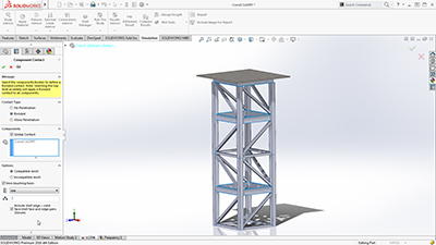
Efficiently optimize and validate each design step using fast-solving, CAD integrated SOLIDWORKS Simulation to ensure quality, performance, and safety.
Tightly integrated with SOLIDWORKS CAD, SOLIDWORKS Simulation solutions and capabilities can be a regular part of your design process—reducing the need for costly prototypes, eliminating rework and delays, and saving time and development costs.
Finite Element Modeling
SOLIDWORKS Simulation uses the displacement formulation of the finite element method to calculate component displacements, strains, and stresses under internal and external loads. The geometry under analysis is discretized using tetrahedral (3D), triangular (2D), and beam elements, and solved by either a direct sparse or iterative solver. SOLIDWORKS Simulation also offers the 2D simplification assumption for plane stress, plane strain, extruded, or axisymmetric options. SOLIDWORKS Simulation can use either an h or p adaptive element type, providing a great advantage to designers and engineers as the adaptive method ensures that the solution has converged.
In order to streamline the model definition, SOLIDWORKS Simulation automatically generates a shell mesh (2D) for the following geometries:
- Sheet metal body—SOLIDWORKS Simulation assigns the thickness of the shell based on the 3D CAD sheet metal thickness, so Product Designers can leverage the 3D CAD data for Simulation purposes.
- Surface body
For shell meshing, SOLIDWORKS Simulation offers a productive tool, called the Shell Manager, to manage multiple shell definitions of your part or assembly document. It improves the workflow for organizing shells according to type, thickness, or material, and allows for a better visualization and verification of shell properties.
SOLIDWORKS Simulation also offers the 2D simplification assumption for plane stress, plane strain, extruded, or axisymmetric options.
Product Engineers can simplify structural beams to optimize performance in Simulation to be modeled with beam elements. Straight, Curved, and tapered Beams are supported. SOLIDWORKS Simulation automatically converts structural members that are created as weldment features in 3D CAD as beam elements for quick setup of the simulation model.
SOLIDWORKS Simulation can use either an h or p adaptive element type, providing a great advantage to designers and engineers, as the adaptive method ensures that the solution has converged. Product Engineers can review the internal mesh elements with the Mesh Sectioning Tools to check the quality of the internal mesh and make adjustments to mesh settings before running the study.
Users can specify local mesh control at vertices, edges, faces, components, and beams for a more accurate representation of the geometry.
Integrated with SOLIDWORKS 3D CAD, finite element analysis using SOLIDWORKS Simulation knows the exact geometry during the meshing process. And the more accurately the mesh matches the product geometry, the more accurate the analysis results will be.
Finite Element Analysis (FEA)
Since the majority of industrial components are made of metal, most FEA calculations involve metallic components. The analysis of metal components can be carried out by either linear or nonlinear stress analysis. Which analysis approach you use depends upon how far you want to push the design:
- If you want to ensure the geometry remains in the linear elastic range (that is, once the load is removed, the component returns to its original shape), then linear stress analysis may be applied, as long as the rotations and displacements are small relative to the geometry. For such an analysis, factor of safety (FoS) is a common design goal.
- Evaluating the effects of post-yield load cycling on the geometry, a nonlinear stress analysis should be carried out. In this case, the impact of strain hardening on the residual stresses and permanent set (deformation) is of most interest.
The analysis of nonmetallic components (such as, plastic or rubber parts) should be carried out using nonlinear stress analysis methods, due to their complex load deformation relationship. SOLIDWORKS Simulation uses FEA methods to calculate the displacements and stresses in your product due to operational loads such as:
- Forces
- Pressures
- Accelerations
- Temperatures
- Contact between components
Loads can be imported from thermal, flow, and motion Simulation studies to perform multiphysics analysis.
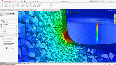
Mesh definition
SOLIDWORKS Simulation offers the capability to mesh the CAD geometry in tetrahedral (1st and 2nd order), triangular (1st and 2nd order), beam, and truss elements. The mesh can consist of one type of elements or multiple for mixed mesh. Solid elements are naturally suitable for bulky models. Shell elements are naturally suitable for modeling thin parts (such as sheet metals), and beams and trusses are suitable for modeling structural members.
As SOLIDWORKS Simulation is tightly integrated inside SOLIDWORKS 3D CAD, the topology of the geometry is used for mesh type:
- Shell mesh is automatically generated for sheet metal model and surface bodies
- Beam elements are automatically defined for structural members
So their properties are seamlessly leveraged for FEA.
To improve the accuracy of results in a given region, the user can define Local Mesh control for vertices, points, edges, faces, and components.
SOLIDWORKS Simulation uses two important checks to measure the quality of elements in a mesh:
- Aspect Ratio Check
- Jacobian Points
In case of mesh generation failure, SOLIDWORKS Simulation guides the users with a failure diagnostics tool to locate and resolve meshing problems. The Mesh Failure Diagnostic tool renders failed parts in shaded display mode in the graphics area.
Subscribe to:
Comments (Atom)